Welcome to MCPlas toolbox!

Introduction
The MCPlas toolbox represents a collection of MATLAB functions for the automated generation of an equation-based fluid-Poisson model for non-thermal plasmas in the multiphysics simulation software COMSOL. Following the development of the new generation of the LXCat platform, all input data are prepared in a structured and interoperable JSON format and can be supplied and validated using existing JSON schemas. The toolbox includes fully transparent, editable MATLAB source code and offers an advanced description of electron transport in addition to commonly used approaches in the plasma modelling community. It supports one-dimensional and two-dimensional modelling geometries employing Cartesian, polar and cylindrical coordinate systems.
The plasma description provided by MCPlas is based on the equations of fluid-Poisson model
\[\begin{split}\frac{\partial}{\partial t}n_j + \nabla\cdot\mathbf{\Gamma}_j = S_j, \label{eq:continuity}\\ % \frac{\partial}{\partial t}w_\mathrm{e} +\nabla\cdot\mathbf{Q}_\mathrm{e} = -e_0\mathbf{\Gamma}_\mathrm{e}\cdot \mathbf{E} + \tilde{S}_\mathrm{e}, \label{eq:we}\\ % -\nabla \cdot(\varepsilon_\mathrm{r}\varepsilon_0\nabla\phi) = \sum_j q_j n_j, \label{eq:poisson}\end{split}\]
where the first equation represents the balance equations for the particle number densities \(n_j\) of species with index \(j\) (electrons, ions, neutrals), charge \(q_j\) and particle flux \(\mathbf{\Gamma}_j\). The second equation is the balance equation for the energy density \(w_\mathrm{e}=n_\mathrm{e}u_\mathrm{e}\) of electrons (\(j = \mathrm{e}\)) with the mean electron energy \(u_\mathrm{e}\) and energy flux \(\mathbf{Q}_\mathrm{e}\). The third equation represents the Poisson equation for the self-consistent determination of the electric potential \(\phi\) and electric field \(\mathbf{E}=-\nabla\phi\). The elementary charge, the relative permittivity of the medium and the vacuum permittivity are denoted by \(e_0\), \(\varepsilon_\mathrm{r}\) and \(\varepsilon_0\), respectively. The source terms \(S_j\) describe the gain and loss of particles due to collision and radiation processes, and \(\tilde{S}_\mathrm{e}\) accounts for the corresponding gain and loss of electron energy. All variables (\(n_j\), \(w_\mathrm{e}\), \(\mathbf{\Gamma}_j\), \(\mathbf{Q}_\mathrm{e}\), \(S_j\), \(\tilde{S}_\mathrm{e}\) and \(\mathbf{E}\)) are space- and time-dependent quantities. To improve clarity and readability, the explicit notation of their dependence on \((\mathbf{r},t)\) is suppressed in the text.
The fluxes \({\mathbf{\Gamma}}_\mathrm{h}\) of heavy particles (\(j=\mathrm{h}\)) are expressed by the common drift-diffusion approximation (Sigeneger, R. Winkler, IEEE Trans. Plasma Sci. 27 (5) (1999) 1254, G. K. Grubert, M. M. Becker, D. Loffhagen, Phys. Rev. E 80 (2009) 036405)
\[\mathbf{\Gamma}_\mathrm{h} = \mathrm{sgn}(q_\mathrm{h})n_\mathrm{h} b_\mathrm{h} \mathbf{E} -D_\mathrm{h}\nabla n_\mathrm{h}\,, \label{eq:flux_particle}\]
where, \(b_\mathrm{h}\) and \(D_\mathrm{h}\) stand for the mobility and diffusion coefficient of heavy species \(\mathrm{h}\), respectively, while the function \(\mathrm{sgn}(q_\mathrm{h})\) defines the sign of \(q_\mathrm{h}\).
Three options are offered by MCPlas for the definition of the electron flux \({\mathbf{\Gamma}}_\mathrm{e}\) and electron energy flux \({\mathbf{Q}}_\mathrm{e}\).
The conventional drift-diffusion approximation (option DDAc) for these fluxes reads
\[\begin{split}\mathbf{\Gamma}_\mathrm{e} = -n_\mathrm{e} b_\mathrm{e} \mathbf{E} -\nabla(D_\mathrm{e}n_\mathrm{e})\,,\label{eq:JeDDAc}\\ % \mathbf{Q}_\mathrm{e} = -w_\mathrm{e} \tilde{b}_\mathrm{e} \mathbf{E} -\nabla(\tilde{D}_\mathrm{e}w_\mathrm{e})\,,\label{eq:QeDDAc}\end{split}\]
where \(b_\mathrm{e}\) and \(D_\mathrm{e}\) are electron transport coefficients, and \(\tilde{b}_\mathrm{e}\) and \(\tilde{D}_\mathrm{e}\) represent the electron energy transport coefficients.
The frequently used approach (option DDA53) employs the simplified form of the electron energy flux
\[\mathbf{Q}_\mathrm{e} = -\frac{5}{3} w_\mathrm{e} {b}_\mathrm{e} \mathbf{E} -\frac{5}{3}\nabla({D}_\mathrm{e}w_\mathrm{e})\,.\label{eq:QeDDA53}\]
The improved drift-diffusion approximation (option DDAn) represents a third way of characterising \({\mathbf{\Gamma}}_\mathrm{e}\) and \({\mathbf{Q}}_\mathrm{e}\).
It was deduced by an expansion of the electron velocity distribution function (EVDF) in Legendre polynomials and the derivation of the first four moment equations from the electron Boltzmann equation (M. M. Becker, D. Loffhagen, AIP Adv. 3 (2013) 012108, M. M. Becker, D. Loffhagen, Adv. Pure Math. 3 (2013) 343).
It reads
\[\begin{split}\mathbf{\Gamma}_\mathrm{e} = -\frac{e_0}{m_\mathrm{e}\nu_\mathrm{e}}\nabla \Bigl((\xi_0 + \xi_2)n_\mathrm{e} \Bigr) -\frac{e_0}{m_\mathrm{e}\nu_\mathrm{e}} \mathbf{E} n_\mathrm{e}\,, \label{eq:JeDDAn}\\ % \mathbf{Q}_\mathrm{e} = -\frac{e_0}{m_\mathrm{e}\tilde{\nu}_\mathrm{e}}\nabla \Bigl((\tilde{\xi}_0 + \tilde{\xi}_2) w_\mathrm{e} \Bigr) \label{eq:QeDDAn}\\ \qquad\qquad\; -\frac{e_0}{m_\mathrm{e}\tilde{\nu}_\mathrm{e}}\Bigl(\frac{5}{3} + \frac{2}{3}\frac{\xi_2}{\xi_0}\Bigr)\mathbf{E} w_\mathrm{e}, \nonumber\end{split}\]
and includes the momentum and energy flux dissipation frequencies \(\nu_\mathrm{e}\) and \(\tilde{\nu}_\mathrm{e}\), respectively, the transport coefficients \(\xi_0\), \(\xi_2\), \(\tilde{\xi}_0\) and \(\tilde{\xi}_2\), as well as electron mass \(m_\mathrm{e}\). It should be emphasized that this approximation is unique to the MCPlas toolbox, as to our knowledge it is not part of any other modelling tool. Considering the accuracy improvements relative to the drift–diffusion approximation at low and atmospheric pressures (M. Baeva, D. Loffhagen, M. M. Becker, D. Uhrlandt Plasma Chem. Plasma Process. 39 (4) (2019) 949–968), it represents a highly significant feature of the toolbox.
Boundary conditions for the electron density and mean electron energy balance equations are included in MCPlas in accordance with the study given by Hagelaar et al. (G. J. M. Hagelaar, F. J. de Hoog, G. M. W. Kroesen, Phys. Rev. E 62 (1) (2000) 1452) and read
\[\begin{split}\mathbf{\Gamma}_\mathrm{e}\cdot\boldsymbol{\nu} = \frac{1-r_\mathrm{e}}{1+r_\mathrm{e}} \Bigl(\left|n_\mathrm{e} \mathbf{v}_{\mathrm{d},\mathrm{e}}\cdot\boldsymbol{\nu} \right| +\frac{1}{2}n_\mathrm{e} v_{\mathrm{th},\mathrm{e}}\Bigr) -\frac{2}{1+r_\mathrm{e}}\gamma\sum_i\max(\mathbf{\Gamma}_i\cdot\boldsymbol{\nu},0) \label{eq:boundary_e}\,,\\ % \mathbf{Q}_\mathrm{e}\cdot\boldsymbol{\nu} = \frac{1-r_\mathrm{e}}{1+r_\mathrm{e}} \Bigl(\left| w_\mathrm{e} \tilde{\mathbf{v}}_{\mathrm{d},\mathrm{e}}\cdot\boldsymbol{\nu} \right| +\frac{2}{3} w_\mathrm{e} v_{\mathrm{th},\mathrm{e}} \Bigr) -\frac{2}{1+r_\mathrm{e}} \gamma u_\mathrm{e}^\gamma \sum_i\max(\mathbf{\Gamma}_i\cdot\boldsymbol{\nu},0)\,,\end{split}\]
where \(\boldsymbol{\nu}\) represents the normal vector pointing toward the plasma boundaries, and \(r_\mathrm{e}\), \(\gamma\), \(u_\mathrm{e}^\gamma\) and \(\mathbf{\Gamma}_i\) denote the electron reflection coefficient, the secondary electron emission coefficient, mean energy of secondary electrons and the ion fluxes at the boundaries, respectively.
The vector of electron drift velocity \(\mathbf{v}_{\mathrm{d},\mathrm{e}}\), the thermal velocity of electron \(v_{\mathrm{th},\mathrm{e}}\), and the vector of electron energy drift velocity \(\tilde{\mathbf{v}}_{\mathrm{d},\mathrm{e}}\) in the case of the conventional drift-diffusion approximation (option DDAc) are defined as
\[\mathbf{v}_{\mathrm{d},\mathrm{e}} = -b_\mathrm{e} \mathbf{E}\, , \qquad % v_{\mathrm{th},\mathrm{e}} = \sqrt{\frac{8 k_\mathrm{B} T_\mathrm{e}}{\pi m_\mathrm{e}}}\, , \qquad % \tilde{\mathbf{v}}_{\mathrm{d},\mathrm{e}} = -\tilde{b}_\mathrm{e} \mathbf{E}\, ,\]
- while in the case of commonly used drift-diffusion approximation (option
DDA53) the vector of electron energy drift velocity \(\tilde{\mathbf{v}}_{\mathrm{d},\mathrm{e}}\) is equal to \(-\frac{5}{3}b_\mathrm{e}\mathbf{E}\). For the improved drift-diffusion approximation (optionDDAn), \(\mathbf{v}_{\mathrm{d},\mathrm{e}}\) and \(\tilde{\mathbf{v}}_{\mathrm{d},\mathrm{e}}\) are defined differently, taking the expressions - \[\begin{split}\mathbf{v}_{\mathrm{d},\mathrm{e}} = -\frac{e_0}{m_\mathrm{e}\nu_\mathrm{e}} \mathbf{E}\, , \qquad %\\ \tilde{\mathbf{v}}_{\mathrm{d},\mathrm{e}} = -\frac{e_0}{m_\mathrm{e}\tilde{\nu}_\mathrm{e}}\Bigl(\frac{5}{3} + \frac{2}{3}\frac{\xi_2}{\xi_0}\Bigr) \mathbf{E}\, . \qquad\end{split}\]
In above relations, \(T_\mathrm{e} = 2u_\mathrm{e}/(3k_\mathrm{B})\) is the temperature of electrons and \(k_\mathrm{B}\) is the Boltzmann constant.
The boundary condition for the balance equation of heavy particle densities has the following form
\[\mathbf{\Gamma}_\mathrm{h}\cdot\boldsymbol{\nu} = \frac{1-r_\mathrm{h}}{1+r_\mathrm{h}} \Bigl(\left|\mathrm{sgn}(q_\mathrm{h}) n_\mathrm{h} \mathbf{v}_{\mathrm{d},\mathrm{h}} \cdot\boldsymbol{\nu}\right| +\frac{1}{2} n_\mathrm{h} {v}_{\mathrm{th},\mathrm{h}} \Bigr), %\]
where the variables and coefficients associated to heavy particles are defined in a manner analogous to that of the electrons.
For the Poisson equation, the boundary conditions are defined by setting the applied voltage \(U_\mathrm{a}\) at the powered electrode and zero potential at the grounded electrode. The accumulation of surface charges is additionally taken into account in the case of dielectric boundaries using the interface condition
\[- \varepsilon_\mathrm{r} \varepsilon_0 \mathbf{E} \cdot \boldsymbol{\nu} = \sigma.\]
Here, \(\varepsilon_\mathrm{r}\) is 1 in the plasma region, while in the dielectric region it has a value characteristic of the considered dielectric. The surface charge density \(\sigma\) is determined from the charged particle currents coming onto the dielectric via equation
\[\frac{\partial \sigma}{\partial t} = \sum_{j}q_j \mathbf{\Gamma}_j \cdot \boldsymbol{\nu}.\]
The source terms \(S_j\) of the electron density balance equations is defined as
\[S_j = \sum_{l=1}^{N_\mathrm{r}} (G_{jl} - L_{jl}) R_l, \label{eq:S_j}\,\]
where \(R_l\) is the reaction rate of reaction \(l\), given by
\[R_l = k_l \prod_{i=1}^{N_\mathrm{s}} n_i^{\beta_{il}}.\]
Here, \(\beta_{il}\) and \(k_l\) denote the partial reaction order of species \(i\) and the rate coefficient for reaction \(l\). \(N_\mathrm{r}\) represents the number of reactions, while \(N_\mathrm{s}\) is the number of species considered in the model. \(G_{jl}\) and \(L_{jl}\) are the gain and loss matrix elements, respectively, defined by the stoichiometric coefficients for the given species and reactions. MCPlas automatically generates these matrices from the RKM input data, which facilitates effortless switching between models with different levels of complexity.
The source terms \(\tilde{S}_\mathrm{e}\) of the electron energy balance equation is defined as
\[\tilde{S}_\mathrm{e} = \sum_{l=1}^{N_\mathrm{r}} \tilde{R}_l,\]
where \(\tilde{R}_l\) is the electron energy rate for reaction \(l\), which is usually defined as reaction rate \(R_l\) multiplied by the net electron energy change (gain or loss) \(\Delta\varepsilon_l\). In the case where electron energy rate coefficient \(\tilde{k}_l\) is defined, e.g.for elastic collision, \(\tilde{R}_l\) is determined as \(\tilde{k}_l \prod_{i=1}^{N_\mathrm{s}} n_i^{\beta_{il}}\). For reactions in which electrons do not participate \(\tilde{R}_l\) is equal to zero.
To ensure numerical stability and obtain consistent solutions, MCPlas uses some stabilisation techniques. One such approach involves the logarithmic transformation of the densities of particle species and the mean electron energy. This inherently enforces positivity and suppresses oscillations in regions with steep gradients or low concentrations The toolbox also implements a source term stabilisation method applicable to all particles and electron energy balance equations, in a similar way to that used in Comsol Plasma Module. This term is designed to counteract numerical instabilities caused by stiff or nonlinear reactions. It acts as a buffer at very low particle number densities, preventing the appearance of negative values, and becomes negligible at higher number densities.
Structure
The code directory has the following structure:
MCPlas
├── applications
│
├── docs
│
├── plasma
│
├── schemas
│
├── toolbox
│
└── MCPlas.m
application
This folder serves as the central location for organizing geometry-specific modeling cases.
It contains subfolders such as Generic1D, Generic1p5D, Generic2D, and Generic2p5D, each corresponding to a particular modelling geometry.
Within each subfolder, there are dedicated MATLAB scripts responsible for defining the geometry, generating the mesh, and configuring project-specific properties such as solvers and study steps.
Each case also includes a General JSON input file that provides essential settings tailored to that specific geometry (options 1D, 1p5D, 2D, 2p5D).
The General JSON input file should be prepared using Adamant web-tool.
How to prepare this input file will be explaned in some of the next sections.
After the model-building process is completed, the resulting .mph file is automatically saved in the same subfolder, keeping all related files organized and localized.
Generic1D
The Generic1D subfolder is dedicated to application of one-dimensional, time-dependent plasma modeling. It contains MATLAB scripts that define the geometry, mesh, and project settings specific to 1D simulations. This modeling case is designed to support plasma source configurations featuring either rectangular or circular electrodes (figure 1), making it suitable for simplified yet physically relevant geometries. The correct specification of electrode dimensions is crucial and must be provided accurately in the associated General JSON input file.
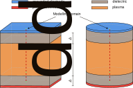
Figure 1, 1D modelling geometry.
Generic1D.mph
General_input_data.json
Generic1p5D
The Generic1p5D subfolder is dedicated to application of one-dimensional, time-dependent plasma modeling in polar coordinates. It contains MATLAB scripts that configure the geometry, meshing, and project settings only for coaxial plasma source configurations (figure 2). This requires that electrode dimensions—such as radius of inner and outer electrodes—be accurately defined in the corresponding General JSON input file. These inputs determine the plasma domain and boundary conditions essential for correct simulation behavior.
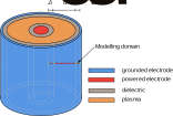
Figure 2, 1p5D modelling geometry for simulations in polar coordiantes.
Generic1p5D.mph
General_input_data.json
Generic2D
The Generic2D subfolder is dedicated to application of two-dimensional, time-dependent plasma modeling in Cartesian coordinates. It contains MATLAB scripts responsible for setting up the geometry, mesh, and project configuration for rectangular electrodes (figure 3). The dimensions and positions of the rectangular electrodes must be properly specified in the associated General JSON input file.
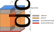
Figure 3, 2D modelling geometry for simulations in Cartesian coordinates.
Generic2D.mph
General_input_data.json
Generic2p5D
The Generic2p5D subfolder is dedicated to the application of two-dimensional, time-dependent plasma modeling in cylindrical coordinates. It contains MATLAB scripts responsible for setting up the geometry, mesh, and project configuration for plasma sources with rectangular or circular electrode shapes (figure 4). The dimensions and positions of both rectangular and circular electrodes must be properly specified in the associated General JSON input file, as they directly affect domain generation and boundary condition assignment.
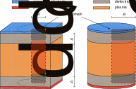
Figure 4, 2D modelling geometry for simulations in cylindrical coordinates.
Generic2p5D.mph
General_input_data.json
docs
All the necessary files for the MCPlas Toolbox documentation are stored in this folder.
plasma
The input data necessary for running MCPlas includes information about the RKM, transport properties of the particle species, as well as general information about the modelling geometry, operating conditions, properties of the plasma source and fluid model properties. These data represent a heterogeneous data set that requires a standardised schema to be verified. MCPlas adopts an extended version of the format proposed by the LXCat platform (open-source) (E. Carbone, W. Graef, G. Hagelaar, D. Boer, M. M. Hopkins, J. C. Stephens, B. T. Yee, S. Pancheshnyi, J. van Dijk, L. Pitchford, Atoms 9 (1) (2021) 1, D. Boer, S. Verhoeven, S. Ali, W. Graef, J. van Dijk, LXCat. URL https://github.com/LXCat-project/LXCat). The basic, top-level structure of the JSON data describing an RKM is shown in figure 5. It comprises three main properties: references; an object storing the references from which included data are extracted, states; an object listing all the states of the particle species considered, and processes; an array of process objects that provide information on the reaction equations and corresponding data. Each individual element of the JSON document is accurately defined by a corresponding JSON schema definition. The exact definition of the LXCat schemas can be found in the LXCat GitHub repository (D. Boer, S. Verhoeven, S. Ali, W. Graef, J. van Dijk, LXCat. URL https://github.com/LXCat-project/LXCat). These schemas can also be used to validate incoming documents. The development of MCPlas has contributed to the extension of the existing electron scattering schemas to further accommodate plasma chemistry data.
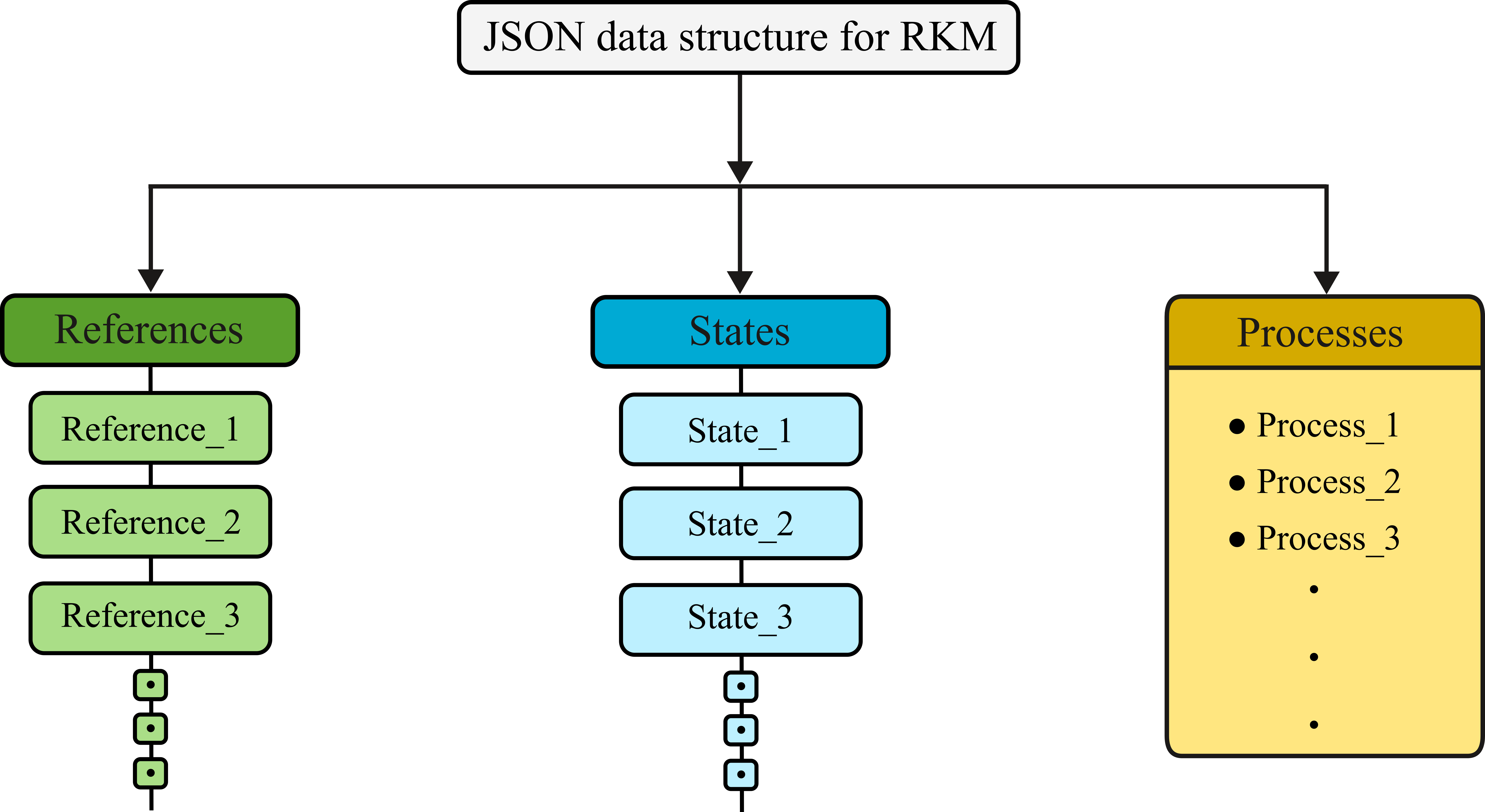
Figure 5, A schematic representing the top-level structure of an LXCat JSON document for LTP input data.
Here are two JSON input data files for argon 4-species and 23-species RKM:
schemas
Inside this folder, you will find the JSON schema used to define general input data via the Adamant web tool. Further details about this file can be found in the Preparation of general input data section.
toolbox
This folder in the MCPlas toolbox contains a collection of MATLAB functions essential for building a COMSOL model using the MATLAB LiveLink module. These functions automate model generation by systematically calling COMSOL-specific commands to define all essential features of the model. By organizing model-building tasks into modular scripts, the folder ensures clarity, maintainability, and flexibility of the model building process.
- ReadJSON
- InpRKM
- InpGeneral
- SetParameters
- SetConstants
- SetVariables
- SetTransportCoefficients
- SetRateCoefficients
- SetEnergyRateCoefficients
- SetRates
- SetEnergyRates
- SetFluxes
- SetSources
- SetProbesAndGraphs
- AddSurfaceChargeAccumulation
- AddPoissonEquation
- AddFluidEquations
- SetElectrical
- SetSelection
- msg
- num2strcell
- IsModelMember
- ActivatePlasma
MCPlas.m
This script serves as the core file of the MCPlas toolbox. It begins by loading user-defined chemistry and general model settings from JSON files, parsing them into structured input objects. After initializing the COMSOL environment and defining the working path, it systematically calls MATLAB functions to establish parameters, geometry, physical constants, variables, transport and reaction coefficients, and model equations. It configures electrical conditions, surface effects, and postprocessing elements like probes and plots. Meshing and solver settings are finalized before the complete model is saved as a .mph file.
Preparation of general input data
In addition to the input data specifying the RKM and the species transport properties, general input data defining the setup are required to build the model. These general input data are provided in the JSON format as well and include information on plasma source, plasma medium, and diagnostics method. The plasma source field describes the geometry, electrical, and material properties of the source. The plasma medium field encompasses the general characteristics of the gas under study, as well as the surface properties specific to the included species and surface materials. Finally, the diagnostics field contains the relevant properties of the fluid-Poisson model, which is employed here as a diagnostic tool for investigation.
For the preparation of the general input data in JSON data format, employing the Adamant tool (https://plasma-mds.github.io/adamant/) for collection of JSON schema-based metadata is proposed. This tool is primarily intended to facilitate the implementation of digital research data management processes by enabling easy compilation and creation of metadata and metadata schemas based on JSON schema standards. All the features of the Adamant are very convenient for generating the JSON data format containing all general input data necessary for model building. In general, Adamant can generate JSON data files based on the included JSON schema. The JSON schema can be included in three ways: (i) selecting one of the existing schemas, (ii) uploading a schema already prepared by the user, or (iii) creating a schema from scratch directly on the platform. The MCPlas toolbox comes with a prepared JSON schema to collect the required general input data based on Plasma-MDS (S. Franke, L. Paulet, J. Schäfer, D. O’Connell, M. M. Becker, Sci. Data (2020) 439), a metadata schema for plasma science. The user has to upload the provided JSON schema to the Adamant platform and start the rendering process. Subsequently, Adamant automatically generates an interactive web-form, whose elements correspond to the general input data that the user has to complete. Compiling the fully defined web-form generates a JSON data file containing all general input data needed for the model building with MCPlas. If the user wants to make a modelling analysis with changed general input data, they just need to generate a modified JSON data file. For the purposes of MCPlas, Plasma-MDS was specifically extended to correspond to the general input data required to set up the fluid-Poisson model in COMSOL. With this, the procedure is designed to promote the further implementation of the FAIR data principles to plasma modelling.
How to use it
MCPlas workflow
The general concept of the MCPlas toolbox is given by the workflow presented in figure 6. At the beginning of the MCPlas workflow, as a first step, all input data necessary for setting up the model must be provided. This considers general input data and plasma chemistry prepared in JSON data format. The second step of the MCPlas workflow involves setting up the model by executing the main MATLAB script, MCPlas.m. This script systematically calls MATLAB functions (listed in section toolbox) specifically designed for the toolbox. The second and third steps automatically execute after running the MCPlas code, and they are not the user’s concern.
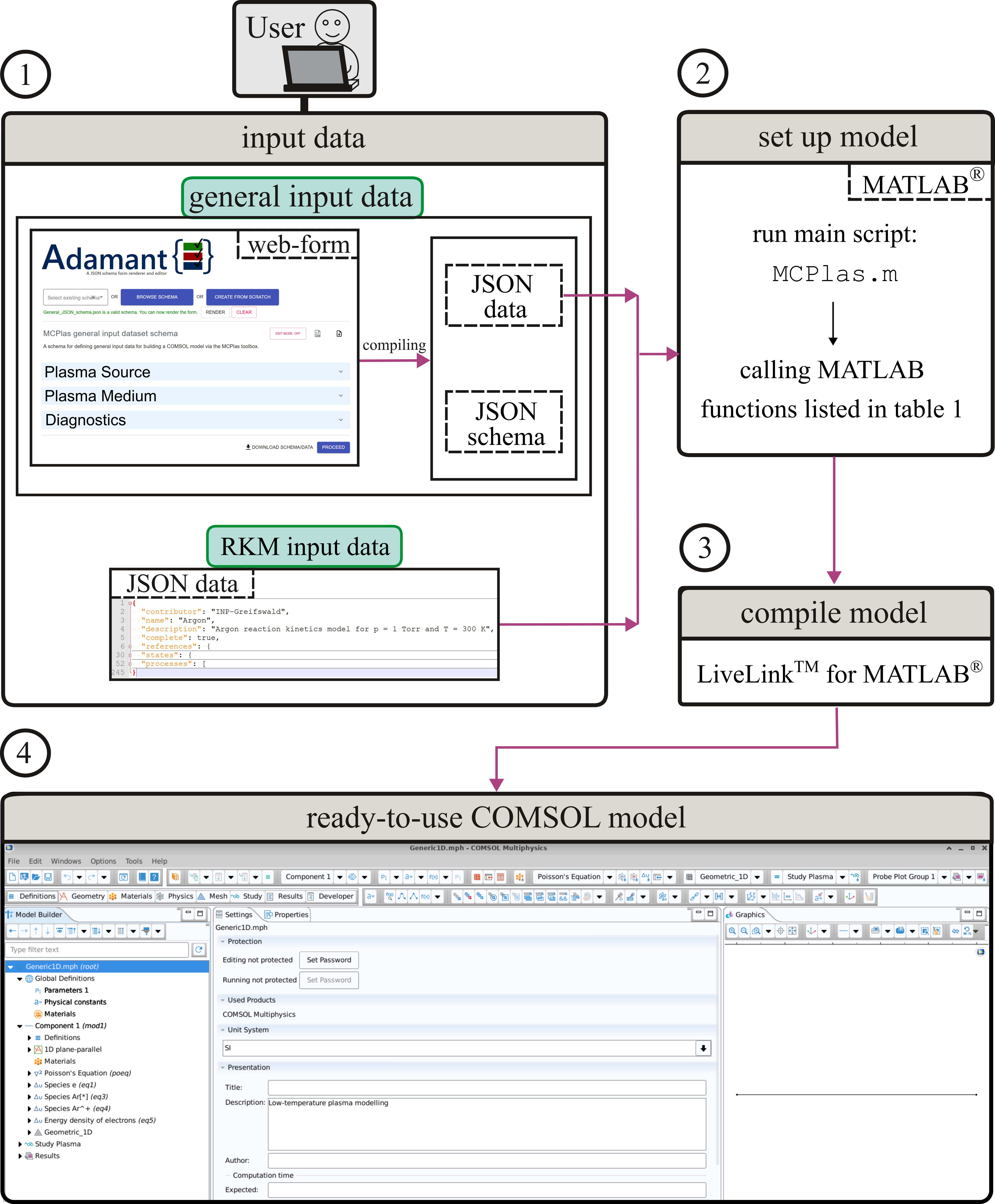
Figure 6, MCPlas worklow.
Step-by-step tutorial
Watch a live demonstration of generating a COMSOL model using MCPlas. The demo covers everything from the initial toolbox setup to generating and running the resulting COMSOL file, with detailed steps and explanations throughout.